The Chern Number
Overview
A Chern number tells us whether something non-trivial is going on in the wavefunction and lets us distinguish between different topological phases.
Now let me clarify what I mean when I say “non-trivial”.
Normally, when we are studying materials, we move from a spatial dependence for the wavefunction to a momentum dependence across a Brillouin Zone.
When we are in a non-trivial phase, we can’t define a wavefunction across the entire Brillouin Zone at the same time. We can rewrite the wavefunction to cover the area that didn’t work before, but then some other section isn’t well-defined.
To be clear, the physics is well defined everywhere, and every way we write the wavefunction gives the same physics. The problem lies in our inability to write down a single “chart” for the whole Zone. This conundrum is similar to the problem with plotting a globe in 2 dimensions. We always have to make cuts, but the entire globe can be covered by “charts” that make up an “atlas”.
Our Model
A page of a Review of Modern Physics behemoth, “Classification of topological quantum matter with symmetries” [1], presented this model below. It inspired me to dig deeper and fill in the details. They attributed this model as describing the Quantum Anomolous Hall Effect, QAHE, but this form describes a wide variety topological phenomena.

 where $\sigma_0$ is the identity matrix and $\sigma_i$ are simply the Pauli matrices.
Combining the terms, $H(k)$ is a 2x2 matrix.
where $\sigma_0$ is the identity matrix and $\sigma_i$ are simply the Pauli matrices.
Combining the terms, $H(k)$ is a 2x2 matrix.
 The wavefunction will then be 2-valued. This could denote two sublattices, or two different types of particles.
While we could use any values for $\vec{R}(k)$, we will use
 as it’s a fairly simple form that gives us the physics we want and exhibits phase transitions depending on the value of $\mu$. I set $\mu$ as $1$ early on. Go through the notebook with that value, then go through the notebook with $\mu = -5, -1, 1, 5$.
using Plots
plotlyjs()
μ=1

labels=["-π","-π/2","0","π/2","π"]
ticks=[-π,-π/2,0,π/2,π];

ks=linspace(-π,π,314)
l=length(ks)

ka=Array{Array{Float64},2}(l,l)
for ii in 1:l
    x=ks[ii]
    for jj in 1:l
        ka[ii,jj]=[x,ks[jj]]
    end
end
function R0(k::Array)
    return 0
end

function R1(k::Array)
    return -2*sin(k[1])
end

function R2(k::Array)
    return -2*sin(k[2])
end

function R3(k::Array)
    return μ+2*cos(k[1])+2*cos(k[2])
end
function R(k::Array)
    return sqrt(R1(k)^2+R2(k)^2+R3(k)^2)
end
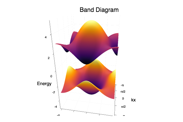
Band Diagram
First, let’s just take a look at the energy spectrum. For each $k$, we calculate the eigenvalues of the 2x2 matrix Hamiltonian.
To make the calculation simpler, I denote the function $R$ as
 With that, energy can simply be written as
 $R_0$ moves the entire spectrum up and down but doesn’t effect the gap, and won’t affect the physics. That term won’t even factor into the eigenvectors.
function λp(k::Array{Float64})
    return R0(k)+R(k)
end

function λm(k::Array{Float64})
    return R0(k)-R(k)
end
Notation Note: I denote the Array evaluation of a function as the function name followed by ‘a’.
λpa=zeros(Float64,l,l)
λma=zeros(Float64,l,l)

for ii in 1:l
    for jj in 1:l
        λpa[ii,jj]=λp(ka[ii,jj])
        λma[ii,jj]=λm(ka[ii,jj])
    end
end
surface(ks,ks,λpa)
surface!(ks,ks,λma)
plot!(xticks= (ticks,labels),
yticks=(ticks,labels),
xlabel="kx",
ylabel="ky",
zlabel="Energy",
title="Band Diagram")
Eigenvectors
To find the eigenvectors, we find the nullspace of the following matrix,

Take the bottom row. Second column value multiples first column and first column value multiples second column.

And now we need to normalize the state
 In low energy, just the minus state will be occupied ,lower energy, but it has a singularity at $\vec{R} = ( 0 ,0, R) $.
We have two complex numbers in this vector, and thus four things to plot $r_1, \theta_1, r_2, \theta_2$,
 But since the eigenvector is only unique up to a phase, we only need to examine the difference in phase, $\theta_1 - \theta_2$.
If we chose to create our vector from the top row instead,
 and normalized
 But the minus state for this one has a singularity at $\vec{R} = (0,0, -R )$.
We can move where the singularity is, but we can’t get rid of it. The problem-point doesn’t show up in the physics, only in the wavefunction representation of it. We cannot well represent the state across the entire Brillouin Zone at the same time. This problem occurs because we have a topologically non-trivial state and a non-zero Chern number.
function up1(k::Array)
    front=1/sqrt(2*R(k)*(R(k)+R3(k)))
    return front*(R(k)+R3(k))
end

function up2(k::Array)
    front=1/sqrt(2*R(k)*(R(k)+R3(k)))
    return front*(R1(k)+im*R2(k))
end

up=Function[]
push!(up,up1)
push!(up,up2)
function um1(k::Array)
    front=1/sqrt(2*R(k)*(R(k)-R3(k)))
    return front*(-R(k)+R3(k))
end

function um2(k::Array)
    front=1/sqrt(2*R(k)*(R(k)-R3(k)))
    return front*(R1(k)+im*R2(k))
end

um=Function[]
push!(um,um1)
push!(um,um2)
upa=zeros(Complex{Float64},2,l,l)
uma=zeros(Complex{Float64},2,l,l)

for ii in 1:l
    for jj in 1:l
        upa[1,ii,jj]=up[1](ka[ii,jj])
        upa[2,ii,jj]=up[2](ka[ii,jj])
        uma[1,ii,jj]=um[1](ka[ii,jj])
        uma[2,ii,jj]=um[2](ka[ii,jj])
    end
end
# Plotting θ2
heatmap(ks,ks,angle.(uma[2,:,:])-angle.(uma[1,:,:]))
plot!(xticks= (ticks,labels),
yticks=(ticks,labels),
xlabel="kx",
ylabel="ky",
title="difference in phase, lower energy")
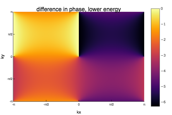
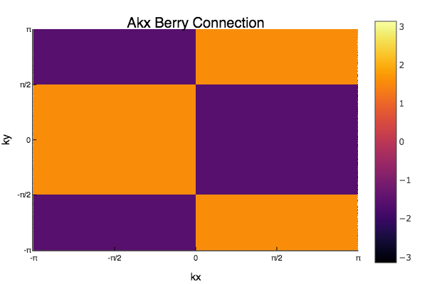
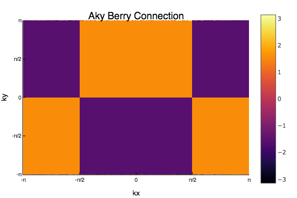
Since eigenvectors are only unique up to a phase, only the relative difference in phase between components is interesting. Notice how there is a singularity where we can't define the phase, and a branch cut where the phase jumps from 0 to $-2\pi$.
surface(ks,ks,norm.(uma[2,:,:]))
plot!(xticks= (ticks,labels),
    yticks=(ticks,labels),
xlabel="kx",
ylabel="ky",
title="magnitude,second component, lower energy")
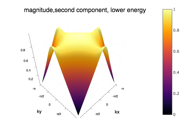
Though this looks smooth throughout the middle, the magnitude does start to behave strangly at the boundries.
surface(ks,ks,norm.(uma[1,:,:]))
plot!(xticks= (ticks,labels),
    yticks=(ticks,labels),
xlabel="kx",
ylabel="ky",
title="magnitude,first component, lower energy")
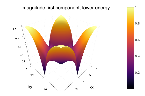
This component is non-differentialable at the origin, as well as four points along the boundary. The phase can be ill defined at the origin only becuase this component goes to zero.
Calculating the Connection
The first step in calculating the Chern number is evaluating the Berry Connection.

Though $\mathcal{A}^i$ looks like a vector, it is not invariant under gauge tranformation. If a wavefunction transforms as
 then the connection transforms as

Near the Dirac points in the Brillouin Zone, the wavefunction has quite a high curvature, which makes the numerical computation of the derivative prone to errors. I tried numerical derivation but was unable to arrive at a correct, stable answer. Therefore, I’m using the ‘ForwardDiff’ Package to take derivatives analytically.
using ForwardDiff
Before dealing with the physics, let’s just look at the syntax for the package.
Here’s just an example of taking the gradient of $x^2$.
ex=x->ForwardDiff.gradient(t->t[1]^2,x)
ex([1])

1-element Array{Int64,1}:
 2
Now let’s apply that syntax to our wavefunctions.
The ‘ForwardDiff’ package seems to only work on purely real functions, so we have to take the derivative of the real and imaginary parts separately.
dum1=kt->ForwardDiff.gradient(um1,kt)

Rdum2=kt->ForwardDiff.gradient(t->real(um2(t)),kt)
Idum2=kt->ForwardDiff.gradient(t->imag(um2(t)),kt)
dum2(k)=Rdum2(k)+im*Idum2(k)
With the derivatives, we can now calculate the connection.
Amkx(k)=conj(um1(k))*dum1(k)[1]+conj(um2(k))*dum2(k)[1]
Amky(k)=conj(um1(k))*dum1(k)[2]+conj(um2(k))*dum2(k)[2]
Akxa=Array{Complex{Float64}}(l,l)
Akya=Array{Complex{Float64}}(l,l)
for ii in 1:l
    for jj in 1:l
        Akxa[ii,jj]=Amkx(ka[ii,jj])
        Akya[ii,jj]=Amky(ka[ii,jj])
    end
end
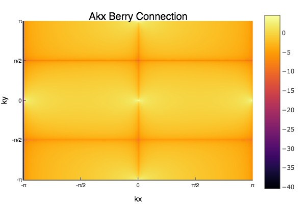
heatmap(ks,ks,log.(norm.(Akxa)))
plot!(xticks= (ticks,labels),
    yticks=(ticks,labels),
xlabel="kx",
ylabel="ky",
title="Akx Berry Connection")
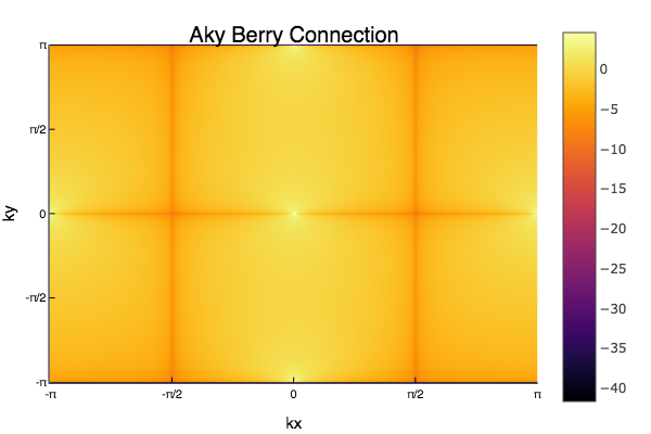
heatmap(ks,ks,log.(norm.(Akya)))
plot!(xticks= (ticks,labels),
    yticks=(ticks,labels),
xlabel="kx",
ylabel="ky",
title="Aky Berry Connection")
heatmap(ks,ks,angle.(Akxa))
plot!(xticks= (ticks,labels),
    yticks=(ticks,labels),
xlabel="kx",
ylabel="ky",
title="Akx Berry Connection")
heatmap(ks,ks,angle.(Akya))
plot!(xticks= (ticks,labels),
    yticks=(ticks,labels),
xlabel="kx",
ylabel="ky",
title="Aky Berry Connection")
Curvature
I previously had a section here about Berry phases, but I need to fix it. Until then, please believe the mass of physics literature that from the guage-dependent Berry connection, we can get a gauge independent quantity called the Berry Curvature. Hopefully I can clarify this mathematical magic when I understand it myself.
Of course it’s called Berry. Every thing in this calculation is named after Berry. At least its not Euler. Done with side note, back to equations.
Here’s our version of Gauss’s Theorem:

And $F_n^{xy}$ will take on this form:


TIME FOR MORE DERIVATIVES!
DRAmkx=kt->ForwardDiff.gradient(t->(real(Amkx(t))),kt )
DImAmkx=kt->ForwardDiff.gradient(t->(imag(Amkx(t))),kt )

DRAmky=kt->ForwardDiff.gradient(t->(real(Amky(t))),kt )
DImAmky=kt->ForwardDiff.gradient(t->(imag(Amky(t))),kt )
F(k)=DRAmky(k)[1]+im*DImAmky(k)[1]-DRAmkx(k)[2]-im*DImAmkx(k)[2]
Fa=Array{Complex{Float64}}(l,l)
for ii in 1:l
    for jj in 1:l
        Fa[ii,jj]=F(ka[ii,jj])
    end
end
maximum(real(Fa))
5.687672555154677e-13
heatmap(ks,ks,imag.(Fa))
plot!(xticks= (ticks,labels),
    yticks=(ticks,labels),
xlabel="kx",
ylabel="ky",
title="Imaginary part of Berry Curvature")
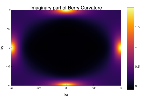
In this situation, the Berry Curvature is a purely imaginary quantity. As you can see in the colorbar, it has both positive and negative areas, but there is an assymtry with much larger positive values. This gives an overall non-zero integral.
Chern Number
Last Step!
Easy calculation now in terms of code, but this number has a great deal of significance. I’m still trying to wrap my head around it. The Chern number seems to pop up in a variety of obscure mathematical stuff over this physicist’s head, but hopefully none of that is necessary to grasp its incredible mind-blowing usefullness.
This single integer not only seperates out topological phases from topologically trivial phases, but seperates different topological phases from each other. And always evaluates to an integer.

If you don’t get approximately an integer, try a finer mesh.
sum(Fa)*(ks[2]-ks[1])^2/(2π*im)
1.0250189329637478 - 9.296489318262423e-34im
Victory !!!!!!!!!!
You made it!
Even if you didn’t understand everything, or really understand much at all, pat yourself on the back. This is the very frontier of science.
[1] Ching Kai Chiu, Jeffrey C.Y. Teo, Andreas P. Schnyder, and Shinsei Ryu, Classification of topological quantum matter with symmetries, Reviews of Modern Physics 88 2016, no. 3, 1–70.
| Topological Physics Series | |||
|---|---|---|---|
| # | Title | Level | Tags |
| 1 | The Chern Number |
||
| 2 | The Winding Number and SSH Model |
||