Computationally Visualizing Crystals
Prerequisites: none
In condensed matter, we find ourselves in the interesting middle ground of dealing with large numbers, e.g. \(10^{23}\), of extremely small particles such as atoms, or electrons.
Luckily, the particles don’t each do their own thing, but often come in nice, structured, repeated units. Lattices. As our first step into the field, we will look at the most basic type, a Bravais lattice.
In a Bravais lattice, every site looks like every other site. Mathematically, we use three vectors, $\vec{a},\vec{b},\vec{c}$ to express how we move from one site to a neighbor.
\begin{equation} \mathbf{R}_{lmn}=l \vec{a} + m \vec{b} + n \vec{c} \;\;\;\; \text{for } l,m,n \in \mathbb{N} \end{equation}
For consistency, we have to put a constraint on these vectors; we cannot combine two of the vectors and obtain the third. If we could, then we couldn’t have sites in an entire three dimensional space.
Stay tuned for a later post where we explore more elaborate lattices.
# importing our packages
using Plots
plotlyjs()
Define The Relevant Variables
Choose the lattice you want to look at, and use that string for the lattice variable. Current options:
- Simple Cubic = “sc”
- Plane triangular lattice = “pt”
- Body-Centered Cubic = “bcc”
- Face-Centered Cubic = “fcc”
Note: Square is Simple Cubic for Nz=1
14 distinct lattice types are possible, but these common four give the important ideas.
Also, input the size of lattice you want to look at.
lattice="fcc";

Nx=3;
Ny=2;
Nz=3;
# A cell to just evaluate
# This one sets the unit vectors (a,b,c) for the different unit cells
# Can you guess what a lattice will look like by looking at the vectors?
if(lattice=="sc")
d=3;
a=[1,0,0];
b=[0,1,0];
c=[0,0,1];
elseif(lattice=="pt")
d=2;
a=[1,0,0];
b=[.5,sqrt(3)/2,0];
c=[0,0,1];
elseif(lattice=="bcc")
d=3;
a=[.5,.5,.5];
b=[.5,.5,-.5];
c=[.5,-.5,.5];
elseif(lattice=="fcc")
d=3;
a=[.5,.5,0];
b=[.5,0,.5];
c=[0,.5,.5];
else
println("Please have a correct lattice")
end# Another cell to just evaluate
N=Nx*Ny*Nz; #The total number of sites
#these allow us to copy an entire row or layer at once
aM=transpose(a);
bM=transpose(repeat(b,outer=[1,Nx]));
cM=transpose(repeat(c,outer=[1,Nx*Ny]));
X=Array{Float64}(undef,N,3); #where we store the positions
"Cell Finished"# Another cell to just evaluate
# Here we are actually calculating the positions for every site
for i in 1:Nx #for the first row
X[i,:]=(i-1)*a;
end
for j in 2:Ny #copying the first row into the first layer
X[Nx*(j-1).+(1:Nx),:]=X[1:Nx,:].+(j-1)*bM;
end
for j in 2:Nz #copying the first layer into the entire cube
X[Ny*Nx*(j-1).+(1:Nx*Ny),:]=X[1:Nx*Ny,:].+(j-1)*cM;
end
Programming Tip:
In Julia, ranges, like 1:Nx, are a special variable type that can be manipulated. We can add numbers to them:
3+(1:3)=4:6,
or add a minus sign to force it to iterate in the opposite direction, though with different start/stop:
-(1:3)=-1:-1:-3
Danger! Make sure to use the parentheses around the range if you are performing these operations.
plot(legend=false,title=lattice,xlabel="X",ylabel="Y",zlabel="Z")

ls=2
v=collect(0:ls)
zed=zeros(length(v))
for ii in 0:ls
    for jj in 0:ls
        plot!(zed .+ii,v,zed .+jj,linecolor=:black)
        plot!(zed .+ii,zed .+jj,v,linecolor=:black)
        plot!(v, zed .+ii,zed .+jj,linecolor=:black)
    end
end

scatter!(X[:,1],X[:,2],X[:,3])
Go Back and Fiddle!
As you might have noticed, this isn’t just a blog where you read through the posts. Interact with it. Change some lines, and see what happens. I choose body centered cubic to display first, but what do the other lattices look like?
Chose pygui(true) to pop open a window and manipulate the plot in 3D.
Look at different lattice sizes.
Can you hand draw them on paper?
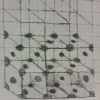
A face centered cubic I decided to draw myself.
Let me know what you think, and enjoy the sequel as well!
| Crystals | |||
|---|---|---|---|
| # | Title | Level | Tags |
| 1 | Computationally Visualizing Crystals |
||
| 2 | Computationally Visualizing Crystals Pt. 2 |
||