Atomic Orbitals

Prerequiresites: Quantum Mechanics course

Electrons around a nucleus. Do they look like little well behaved planets orbiting a sun?

NOPE!

We get spread out blobs in special little patterns called orbitals. Here, we will look at their shapes and properties a bit. Today we will look at graphs in 1D and 2D, but the next post, Atomic Orbitals Pt. 2, uses a fancy, but slightly unstable plotting package, GLVisualize to generate some 3D plots.

The Hamiltonian for our problem is:

\begin{equation} {\cal H}\Psi(\mathbf{x}) =\left[ -\frac{\hbar}{2 m} \nabla^2 - \frac{Z e^2}{4 \pi \epsilon_0 r}\right]\Psi(\mathbf{x}) = E \Psi(\mathbf{x}) \end{equation} with \begin{equation} \nabla^2= \frac{1}{r^2}\frac{\partial}{\partial r} \left( r^2 \frac{\partial}{\partial r} \right)+ \frac{1}{r^2 \sin \theta} \frac{\partial}{\partial \theta} \left( \sin \theta \frac{\partial}{\partial \theta} \right)+ \frac{1}{r^2 \sin^2 \theta} \frac{\partial^2}{\partial \phi^2} \end{equation}

To solve this problem, we begin by guessing a solution with separated radial and angular variables, \begin{equation} \Psi(\mathbf{x}) = R(r) \Theta ( \theta,\phi) \end{equation}

\begin{equation} \frac{E r^2 R(r)}{2r R^{\prime}(r) + r^2 R^{\prime \prime}(r)}= \frac{\left( \frac{1}{\sin \theta} \frac{\partial}{\partial \theta} \left( \sin \theta \frac{\partial \Theta(\theta,\phi)}{\partial \theta} \right)+ \frac{1}{\sin^2 \theta} \frac{\partial^2 \Theta(\theta,\phi)}{\partial \phi^2}\right) }{\Theta( \theta, \phi)} =C \end{equation}

Instead of going into the precise mechanisms of solving those two separate equations here, trust for now that they follow standard special functions, the associated Legendre polynomial and the generalized Laguerre polynomial. Try a standard quantum mechanics textbook for more information about this.

\begin{equation} Y^m_l(θ,ϕ) = (-1)^m e^{i m \phi} P^m_l (\cos(θ)) \end{equation} where $P^m_l (\cos (\theta))$ is the associated Legendre polynomial.

\begin{equation} R^{n,l} ( \rho ) = \rho ^l e^{- \rho /2} L^{2 l+1}_{n-l-1} ( \rho ) \end{equation} where $L^{2 l+1}_{n-l-1}(\rho)$ is the generalized Laguerre polynomial.

\begin{equation} \rho=\frac{2r}{n a_0} \end{equation}

\begin{equation} N=\sqrt{\left(\frac{2}{n}\right)^3 \frac{(n-l-1)}{2n(n+l)!}} \end{equation}

#Pkg.update();
#Pkg.add("GSL");
#Pkg.add("PyPlot");
using GSL;    #GSL holds the special functions
using PyPlot;

Cell to Evaluate

What’s below is a bunch of definitions that makes our calculations easier later on. Here I utilize the GNU scientific library, GSL imported above, to calculate the special functions.

a0=1; #for convenience, or 5.2917721092(17)×10−11 m

# The unitless radial coordinate
ρ(r,n)=2r/(n*a0);

#The θ dependence
function Pmlh(m::Int,l::Int,θ::Real)
    return (-1.0)^m *sf_legendre_Plm(l,m,cos(θ));
end

#The θ and ϕ dependence
function Yml(m::Int,l::Int,θ::Real,ϕ::Real)
    return  (-1.0)^m*sf_legendre_Plm(l,m,cos(θ))*e^(im*m*ϕ)
end

#The Radial dependence
function R(n::Int,l::Int,ρ::Real)
    if isapprox(ρ,0)
        ρ=.01
    end
     return sf_laguerre_n(n-l-1,2*l+1,ρ)*e^(-ρ/2)*ρ^l
end

#A normalization: This is dependent on the choice of polynomial representation
function norm(n::Int,l::Int)
    return sqrt((2/n)^3 * factorial(n-l-1)/(2n*factorial(n+l)))
end

#Generates an Orbital function of (r,θ,ϕ) for a specified n,l,m.
function Orbital(n::Int,l::Int,m::Int)
    if l>n    # we make sure l and m are within proper bounds
        throw(DomainError())
    end
    if abs(m)>l
        throw(DomainError())
    end
    psi(ρ,θ,ϕ)=norm(n, l)*R(n,l,ρ)*Yml(m,l,θ,ϕ);
    return psi
end

#We will calculate is spherical coordinates, but plot in Cartesian, so we need this array conversion
function SphtoCart(r::Array,θ::Array,ϕ::Array)
    x=r.*sin(θ).*cos(ϕ);
    y=r.*sin(θ).*sin(ϕ);
    z=r.*cos(θ);
    return x,y,z;
end

function CarttoSph(x::Array,y::Array,z::Array)
    r=sqrt(x.^2+y.^2+z.^2);
    θ=acos(z./r);
    ϕ=atan(y./x);
    return r,θ,ϕ;
end

"Defined Helper Functions"

Parameters

Grid parameters: You might need to change rmax to be able to view higher $n$ orbitals.

Remember that \begin{equation} 0<n \;\;\;\;\; \;\;\;\; 0 \leq l < n \;\;\;\;\; \;\;\;\; -l \leq m \leq l \;\;\;\;\; \;\;\;\; n,l,m \in {\cal Z} \end{equation}

# Grid Parameters
rmin=.05
rmax=10
Nr=100 #Sampling frequency
Nθ=100
Nϕ=100

# Choose which Orbital to look at
n=3;
l=1;
m=0;
"Defined parameters"

#Linear Array of spherical coordinates
r=collect(linspace(rmin,rmax,Nr));
ϕ=collect(linspace(0,2π,Nθ));
θ=collect(linspace(0,π,Nϕ));
#3D arrays of spherical coordinates, in order r,θ,ϕ
ra=repeat(r,outer=[1,Nθ,Nϕ]);
θa=repeat(transpose(θ),outer=[Nr,1,Nϕ]);
ϕa=repeat(reshape(ϕ,1,1,Nϕ),outer=[Nr,Nθ,1]);

x,y,z=SphtoCart(ra,θa,ϕa);

Though I could create a wrapped up function with Orbital(n,l,m) and evaluate that at each point, the below evaluation takes advantage of the separability of the solution with respect to spherical dimensions. The special functions, especially for higher modes, take time to calculate, and the fewer calls to GSL, the faster the code will run. Therefore, this implementation copies over radial and angular responses.

Ψ=zeros(Float64,Nr,Nϕ,Nθ)
θd=Int64(round(Nθ/2))  ## gives approximately the equator.  Will be useful later

p1=Pmlh(m,l,θ[1]);
p2=exp(im*m*ϕ[1]);
for i in 1:Nr
    Ψ[i,1,1]=norm(n,l)*R(n,l,ρ(r[i],n))*p1*p2;
end

for j in 1:Nθ
    Ψ[:,j,1]=Ψ[:,1,1]*Pmlh(m,l,θ[j])/p1;
end

for k in 1:Nϕ
    Ψ[:,:,k]=Ψ[:,:,1]*exp(im*m*ϕ[k])/p2;
end

pygui(false)
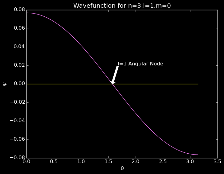
xlabel("θ")
ylabel("Ψ")
title("Wavefunction for n= $n ,l= $l ,m= $m ")

annotate("l= $l Angular Node",
xy=[π/2;0],
xytext=[π/2+.1;.02],
xycoords="data",
arrowprops=Dict("facecolor"=>"black"))

plot(θ,zeros(θ))
plot(θ,reshape(Ψ[50,:,1],100)) #reshape makes Ψ 1D

A slice along the θ plane showing an angular node for the 2p orbital.

pygui(false)
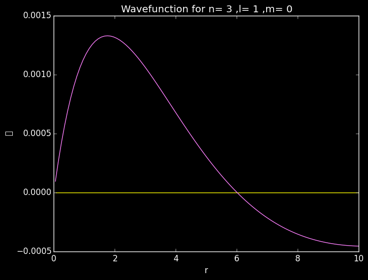
xlabel("r")
ylabel("Ψ")
title("Wavefunction for n= $n ,l= $l ,m= $m ")

plot(r,zeros(r))
plot(r,reshape(Ψ[:,50,1],100)) #reshape makes Ψ 1D

A slice along the radial plane showing a radial node in the 3p orbital.

#rap=squeeze(ra[:,:,50],3)
#θap=squeeze(θa[:,:,50],3)
#ϕap=squeeze(ϕa[:,:,50],3)
#Ψp=squeeze(Ψ[:,:,50],3)
rap=ra[:,:,50]
θap=θa[:,:,50]
ϕap=ϕa[:,:,50]
Ψp=Ψ[:,:,50]
xp,yp,zp=SphtoCart(rap,θap,ϕap);
pygui(false)
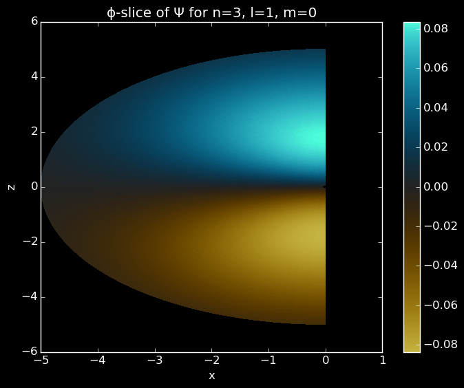
xlabel("x")
ylabel("z")
title("ϕ-slice of Ψ for n=$n, l=$l, m=$m")
pcolor(xp[:,:],zp[:,:],Ψp[:,:],cmap="coolwarm")
colorbar()

Slice of a 3p orbital in the x and z plane.

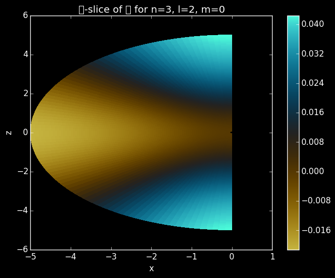
Slice of a 3dz2 orbital in the x and z plane.

Don’t forget to check out Atomic Orbitals Pt. 2!