I wrote this piece as part of a presentation I gave to the robotics team at Benson High School in Portland, OR. My thanks to my mentor John Delacy for working with me in high school and fostering my love for science and astronomy, and for inviting me to help work with the next generation of scientists and engineers. I loved getting to see their robots and hear about the competitions.

Intro to Jupyter Notebooks

Currently we are using a jupyter notebook. This format can support either Julia, Python, or R. The format is quite similiar to that used in the propriety software Mathematica.

We have two types of cells:

• Markdown cells
• Code Cells

Markdown Cells

This is a Markdown Cell. Here we write text or add pictures to describe what we are doing. In raw format, everything is easily readable, but the computer can also render it to look even nicer with headings, lists,bold,italic, tables, links, and other formatting.

I can even write equations.

Equations use LaTeX syntax. LaTeX is a document preparation language used by those in STEM. It’s how we make all those awesome looking papers. It also automatically handles our citations for us :) Check out Overleaf to create documents online.

I can also write code inline x+=1 or in block style

for ii in 1:n
    x+=1
end

Coding Cells

You can evaluate coding cells by pushing Shift-Enter.

Next to Coding Cells, In[ ] specifies the code that will be executed, and Out[] specifies the output of the given cell. The number specifies the order in which the code got evaluated.

Important: Global variables get edited each time you evaluate a new cell. So order of evaluation matters.

Julia’s Packages

Julia uses external packages, much like Python, to supplement its core functionality. PyPlot imports plotting functionality from Python’s PyPlot with the package PyCall. Julia maintains a complete list of supported external packages. While many are quite specialized or out of date, some are incredibly useful, like different plotting tools, curve fitting, integrators, differential equations, accelerators, working with different file types, and more.

If you need to run a jupyter notebook on your machine instead of on JuliaBox, you would be using the IJulia package.

# Update packages
Pkg.update()

# Add a new package to your repository
# Unnecessary if already added
#Pkg.add("PyPlot")

# Load PyPlot into
using PyPlot

Projectile Motion

An example of a projectile.

BUT

NO! How do we solve this?

First let’s write down the infinitesimal, exact version of the equations. Sorry if you haven’t had Calculus yet. Just block out this part and keep going.

In order to put this into an equation, we take the derivative and break it into a courser grained version

Now because $\Delta x$ and $\Delta t$ have actual sizes instead of being infinitesimally small, the computer can deal with them.

Now we take lots of baby steps of $\Delta t$ over our time interval to change the position with the changing velocity.

We can also think of this as finding a small enough interval such that we can treat the y velocity as if it’s constant.

Bonus note: Different types of algorithms,like symplectic, evaluate the velocity at different time points.

A cell of parameters we need to enter

This first cell is parameters that we need to decided upon. I’ve put in numbers that are fairly resonable and tested.

You can change the value of them and see what happens to the final answer. Hopefully nothing will break ;)

θ=π/4 #angle with respect to horizontal
v0=10 # intial velocity

x0=0; # initial position
y0=0;

t0=0 #initial time
tf=2 #final time
dt=1e-3 #time step size

Preliminary calculation of important variables

This is again more parameters, but this cell shouldn’t be changed.

Unless you want to go to the moon or Mars…

g=9.8 #m/s^2

vx0=v0*cos(θ) # x component of velocity at initial time step
vy0=v0*sin(θ) # y component of velocity at initial time step

t=collect(t0:dt:tf) # creates an array that holds each time point
nt=length(t) #the number of time steps we willl have

Initialization of Variables

As we march along for a bunch of time steps, we will be computing our position and velocity, but we will need some place to put those numbers. It’s more efficient and better practice to create a place to put those numbers beforehand. So that’s what we are doing here.

We are also setting the first value in the position/ velocity vectors to be their initial values.

#initializing empty vectors that will hold position and velocity at each time step
x=zeros(t)
y=zeros(t)
vx=zeros(t)
vy=zeros(t)

x[1]=x0
y[1]=y0
vx[1]=vx0
vy[1]=vy0

Loop of Time Steps

Now we do our actual calculation. We march along, taking tiny little baby steps, calculating our new positions and our new velocities and storing them in our vectors.

for ii in 2:nt
    x[ii]=x[ii-1]+vx[ii-1]*dt
    y[ii]=y[ii-1]+vy[ii-1]*dt

    vx[ii]=vx[ii-1]
    vy[ii]=vy[ii-1]-g*dt
end

Plotting

We use PyPlot to display our results here. It’s imported into Julia from Python and has great documentation and versitility.

plot(x,y)

xlabel("x")
ylabel("y")
title("Simple Projectile Motion")

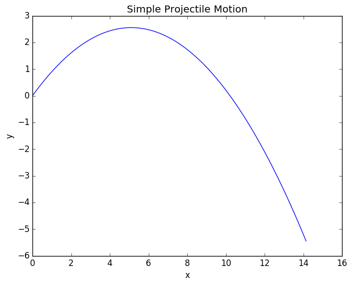
Simple Projectile Motion.

yexact=-g/2.*t.^2.+vy0.*t

plot(t,y,linewidth=6,label="Numerical")
plot(t,yexact,label="Exact")

xlabel("t")
ylabel("y")
legend()
title("Comparing Numerical and Exact Calculations")

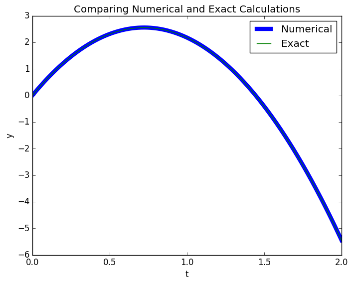
Comparing Numerical and Exact Calculations

plot(t,yexact-y)

xlabel("t")
ylabel("Y Error")
title("Error over time of Numerical solution at dt= $dt")

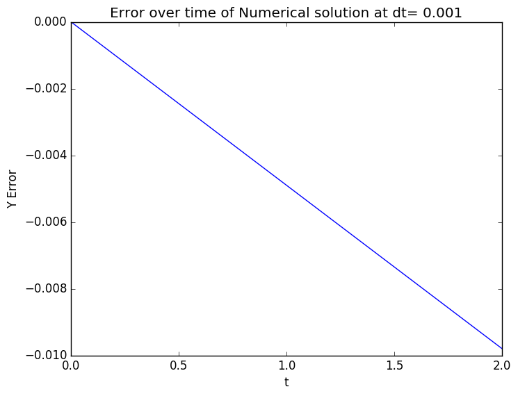
Error over time of Numerical Solution

plot(t,vy,label="vy")
plot(t,vx,label="vx")

xlabel("t")
ylabel("velocity")
legend()
title("Velocities over time")

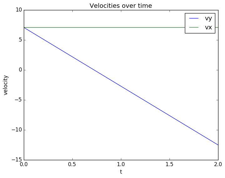
Velocity Evolution. Notice how the x velocity remains constant while the y velocity accelerates.

But what if there is a surface?

If we place a surface at $y=0$, or any other location, the ball won’t just keep on falling forever. We can choose two types of actions when it encounters the surface

• Elastic Collision: The ball bounces with the same amount of kinetic energy, just in the opposite direction
• Inelastic Collision: The ball looses a fraction of its energy in the collision.
  • At an extreme of this case, the ball looses all its energy.

We use an if statement to determine when it encounters the surface. We’ll just do an elastic collision, so we can just change $v_y$ and not have to worry about total energy, etc.

for ii in 2:nt
    x[ii]=x[ii-1]+vx[ii-1]*dt
    y[ii]=y[ii-1]+vy[ii-1]*dt

    if y[ii]<0
        println("Hit the surface at t: ",t[ii],"\t x: ",x[ii])
        vy[ii-1]=-vy[ii-1]
        y[ii]=y[ii-1]+vy[ii-1]*dt
    end

    vx[ii]=vx[ii-1]
    vy[ii]=vy[ii-1]-g*dt
end

Hit the surface at t: 1.445	 x: 10.217692988145673

plot(x,y)

xlabel("x")
ylabel("y")

title("Projectile Motion with a Surface")

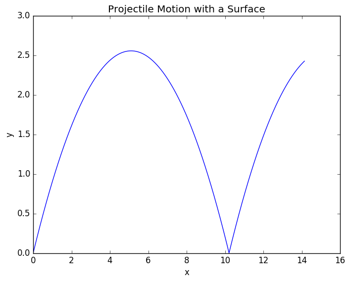
Projectile with surface. Notice it bounce at x=10.2

plot(t,vy,label="vy")
plot(t,vx,label="vx")

xlabel("t")
ylabel("velocity")
legend()
title("Velocity over time with bounce")

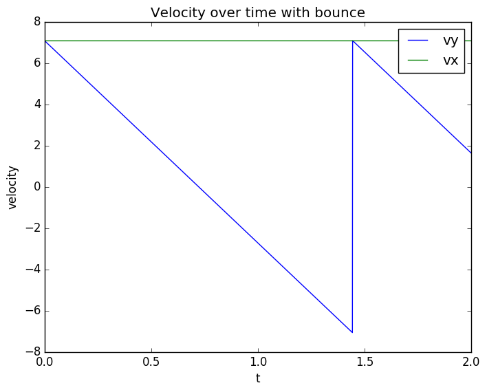
Velocity with Bounce. At t=1.445, the y velocity switches to positive.

Why do we do analytics at all?

So we just found our intercepts and made a bunch of nice graphs without ever having to do any algebra. Why do we force you to slog through it?

Because you need to know what to expect to know when it’s completely going wrong or when something might fail numerically.

This problem is pretty robust, but if you try other problems like the Van der Pol problem, or one’s that display any instability or chaos, we would really need to callibrate to the right time step size. More specialized algorithms, like the ones I talk about in my ODE post, also allow you more accuracy for larger step sizes.

Let’s do the same things but for a range of different time steps to show some of the limitations of numerical analysis.

# Lets choose our step sizes
dta=[.001,.01,.1,.2]

4-element Array{Float64,1}:
 0.001
 0.01
 0.1
 0.2

# The length of each time series
# All arrays will be the same length, but some will be padded
na=floor(Int,(tf-t0)./dta)

# The place holding arrays
ta=zeros(Float64,maximum(na),length(dta))
xa=zeros(ta)
ya=zeros(ta)
vxa=zeros(ta)
vya=zeros(ta)

# Where we start
xa[1,:]=x0
ya[1,:]=y0
vxa[1,:]=vx0
vya[1,:]=vy0

# We perform one loop for each step size
for jj in 1:length(dta)

    # This is the step size for the loop
    dt=dta[jj]
    # We only use the first na[jj] of the arrays
    ta[1:na[jj],jj]=linspace(t0,tf,na[jj])

    #The same loop we had before
    for ii in 2:na[jj]
        xa[ii,jj]=xa[ii-1,jj]+vxa[ii-1,jj]*dt
        ya[ii,jj]=ya[ii-1,jj]+vya[ii-1,jj]*dt

        if ya[ii,jj]<0
            vya[ii-1,jj]=-vya[ii-1,jj]
            ya[ii,jj]=ya[ii-1,jj]+vya[ii-1,jj]*dt
        end

        vxa[ii,jj]=vxa[ii-1,jj]
        vya[ii,jj]=vya[ii-1,jj]-g*dt
    end

end

for ii in 1:length(dta)
    plot(xa[1:na[ii],ii],ya[1:na[ii],ii],label=dta[ii])
end

xlabel("x")
ylabel("y")
legend()
title("Projectile Motions for different time step sizes")

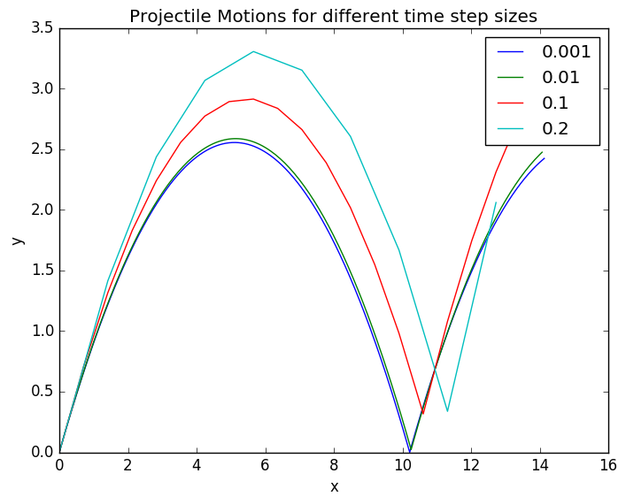
Projectile Approximations for different step sizes. As we take larger step sizes, our approximations get successively worse.

yexact=-g/2.*ta.^2.+vy0.*ta
yerr=ya-yexact
ylim(-.5,4)

for ii in 1:length(dta)
    plot(ta[1:na[ii],ii],yerr[1:na[ii],ii],label=dta[ii])
end

annotate("The Bounce",
    xy=[1.5, 1.4 ],
    xytext=[.5, 1.5],
   xycoords="data",
   arrowprops=Dict("facecolor"=>"green"))

xlabel("time")
ylabel("y error")
legend()
title("Error in y position for different time step sizes")

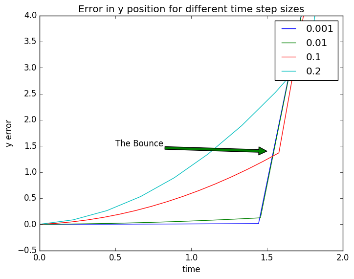
Error from the exact solution for each of our approximations. The exact equation doesn't have a bounce, so we just take the error up to that point.

But what about Air Resistence?

Real objects encounter air resistence proportional to velocity. This can’t be solved analytically, but our code can handle it really easily.

R=.01
dt=1e-3

t=collect(t0:dt:tf) # creates an array that holds each time point
nt=length(t) #the number of time steps we willl have

#initializing empty vectors that will hold position and velocity at each time step
x=zeros(t)
y=zeros(t)
vx=zeros(t)
vy=zeros(t)

x[1]=x0
y[1]=y0
vx[1]=vx0
vy[1]=vy0

E=zeros(t)
E[1]=.5*(vx0^2+vy0^2)

for ii in 2:nt
    x[ii]=x[ii-1]+vx[ii-1]*dt
    y[ii]=y[ii-1]+vy[ii-1]*dt

     if y[ii]<0
        #println("Hit the surface at t: ",t[ii],"\t x: ",x[ii])
        vy[ii-1]=-vy[ii-1]
        y[ii]=y[ii-1]+vy[ii-1]*dt
    end

    sc=sqrt(vx[ii-1]^4+vy[ii-1]^4)/sqrt(vx[ii-1]^2+vy[ii-1]^2)
    vx[ii]=vx[ii-1]-R*vx[ii-1]*sc*dt
    vy[ii]=vy[ii-1]-g*dt-R*vy[ii-1]*sc*dt

    E[ii]=g*y[ii]+.5*(vx[ii]^2+vy[ii]^2)
end

plot(x,y)

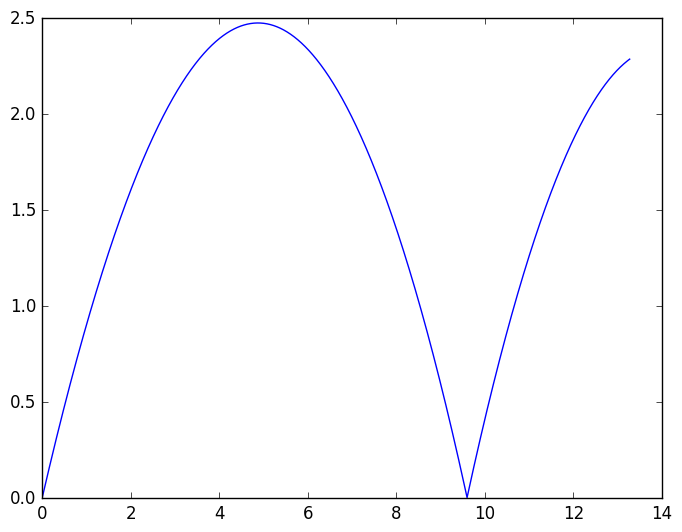
Path of projectile in the presence of air resistance.

yexact=-g/2.*t.^2.+vy0.*t

plot(t,y,label="Air Resistence")
plot(t,yexact,label="Exact No Air")
ylim(-.5,3)

xlabel("t")
ylabel("y")
legend()
title("Comparing With and Without Air")

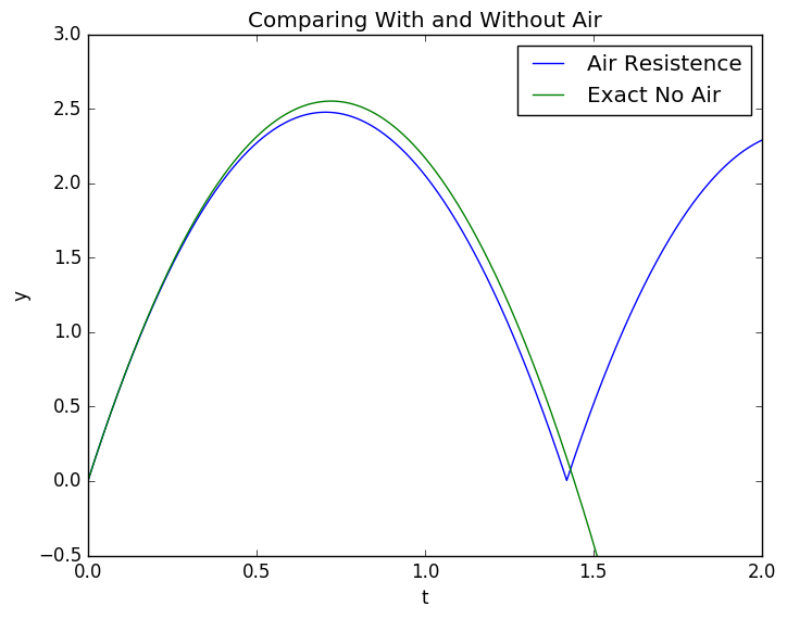
Here we compare the height with and without air resistance over time. The ball doesn't go quite as high and falls a little sooner.

plot(t,vy)

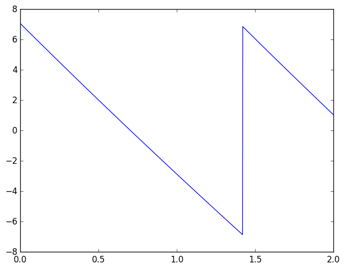
Y Velocity with Drag

plot(t,vx)

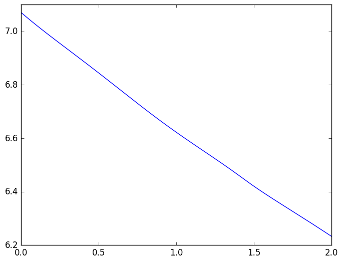
X Velocity with Drag. Here we can see that the projectile slows down in the x direction instead of remaining at the at the same speed like in the other cases, since we have added a force in the x-direction.

plot(t,E)

xlabel("time")
ylabel("Energy")
title("Decaying Energy with Air Resistence")

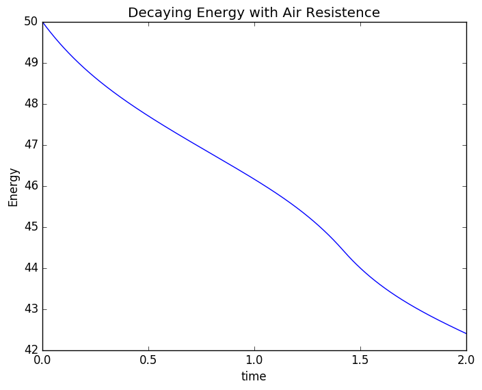
Energy Decay. The drag takes energy out of the projectile and disperses into heat. We lose energy from the potential + kinetic energy sum that we can't get back.

Terminal Velocity

Since we already have the piece of code for air resistance written, let’s just run it for a freely falling object to determine terminal velocity.

tf=10

t=collect(t0:dt:tf) # creates an array that holds each time point
nt=length(t) #the number of time steps we will have

#initializing empty vectors that will hold position and velocity at each time step
y=zeros(t)
vy=zeros(t)
E=zeros(t)

y[1]=0
vy[1]=0

E[1]=.5*vy0^2

for ii in 2:nt
    y[ii]=y[ii-1]+vy[ii-1]*dt

    vy[ii]=vy[ii-1]-g*dt-R*sign(vy[ii-1])*vy[ii-1]^2*dt

    E[ii]=g*y[ii]+.5*vy[ii]^2
end

plot(t,vy,label="Velocity")
plot(t,vy[end]*ones(t),label=round(vy[end],2))

xlabel("time")
ylabel("y velocity")
legend()
title("Approaching terminal velocity")

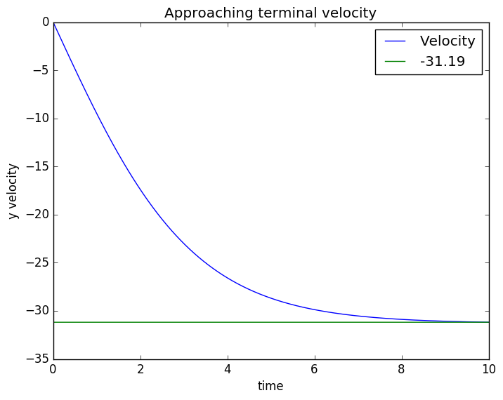
A freely falling ball approaching terminal velocity. After 10 time, it reaches -31.19 dist/time with little acceleration.

plot(t,y)
xlabel("time")
ylabel("Position")
title("Particle Falling in Air Resistence")

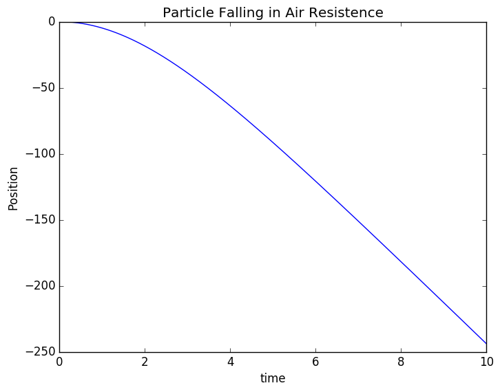
In the beginning, the particles path looks like a parabola, but as it reaches high speed, the path starts to better mimic a straight line.

plot(t,E)
xlabel("time")
ylabel("Energy")
title("Energy of Falling Particle")

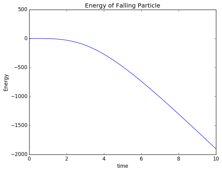
As this projectile hits no surface, it can constantly convert gravitational potential to kinetic energy to heat, with nothing stopping it. Thus it ends up losing energy at a linear rate in the steady state.

The Termination

Now that we have see terminal velocity, I will terminate this post. See you next time :)